Increasing the efficiency of labor increases the supply of labor measured in efficiency units. An increase in labor efficiency means that the same amount of labor can produce higher output. It also reduces the demand for other factors through substitution effects. In this experiment, labor efficiency is increased permanently by 1 percent. (See experiment)
Table 12. The effect of a permanent increase in labor efficiency
| 1. yr | 2. yr | 3. yr | 4. yr | 5. yr | 10. yr | 15. yr | 20. yr | 25. yr | 30. yr | ||
| Million 2005-kr. | |||||||||||
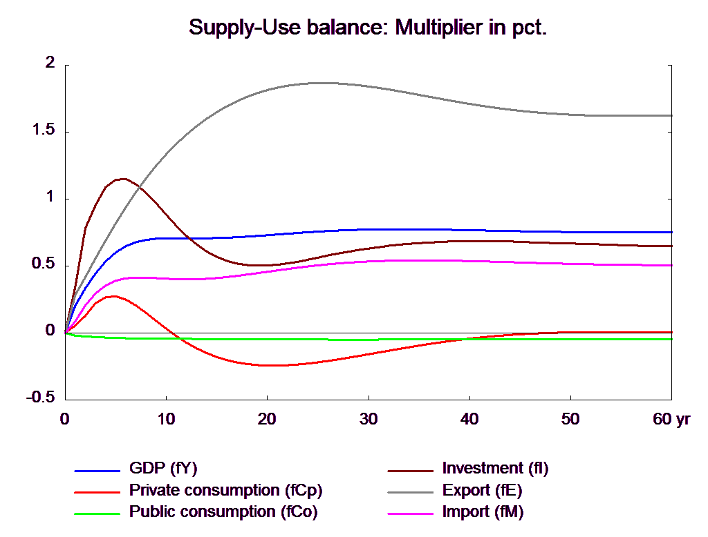
| Priv. consumption | fCp | 439 | 1020 | 1799 | 2186 | 2279 | 286 | -1738 | -2530 | -2456 | -1917 |
| Pub. consumption | fCo | -82 | -107 | -129 | -147 | -161 | -201 | -229 | -260 | -289 | -313 |
| Investment | fI | 1181 | 2639 | 3359 | 3911 | 4196 | 3525 | 2453 | 2346 | 2822 | 3409 |
| Export | fE | 2532 | 3802 | 5169 | 6487 | 7820 | 13737 | 18288 | 21663 | 24005 | 25512 |
| Import | fM | 737 | 1818 | 2677 | 3278 | 3675 | 4124 | 4501 | 5400 | 6428 | 7319 |
| GDP | fY | 3227 | 5265 | 7100 | 8659 | 9900 | 12554 | 13562 | 15050 | 16815 | 18469 |
| 1000 Persons | |||||||||||
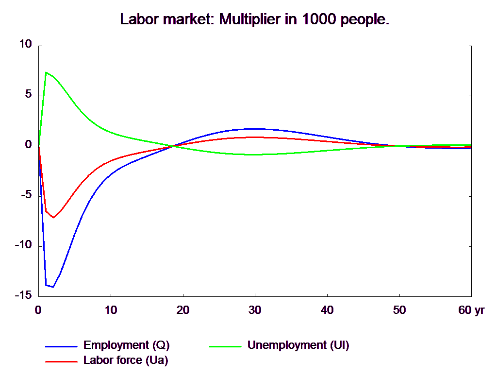
| Employment | Q | -13.85 | -14.04 | -12.66 | -10.73 | -8.74 | -2.82 | -1.00 | 0.35 | 1.37 | 1.71 |
| Unemployment | Ul | 7.36 | 6.91 | 6.16 | 5.19 | 4.21 | 1.36 | 0.48 | -0.18 | -0.68 | -0.84 |
| Percent of GDP | |||||||||||
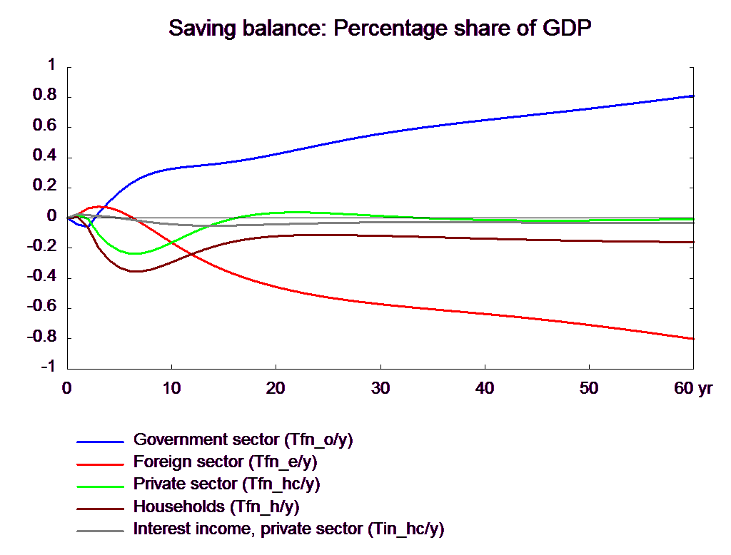
| Pub. budget balance | Tfn_o/Y | -0.04 | -0.06 | 0.03 | 0.11 | 0.17 | 0.33 | 0.36 | 0.42 | 0.49 | 0.56 |
| Priv. saving surplus | Tfn_hc/Y | 0.02 | -0.01 | -0.11 | -0.18 | -0.22 | -0.16 | -0.02 | 0.03 | 0.03 | 0.01 |
| Balance of payments | Enl/Y | -0.02 | -0.06 | -0.08 | -0.07 | -0.05 | 0.16 | 0.34 | 0.46 | 0.53 | 0.57 |
| Foreign receivables | Wnnb_e/Y | 0.30 | 0.35 | 0.34 | 0.32 | 0.31 | 0.81 | 2.10 | 3.74 | 5.46 | 7.13 |
| Bond debt | Wbd_os_z/Y | 0.25 | 0.33 | 0.30 | 0.22 | 0.07 | -1.10 | -2.38 | -3.70 | -5.10 | -6.56 |
| Percent | |||||||||||
| Capital intensity | fKn/fX | -0.23 | -0.34 | -0.42 | -0.47 | -0.50 | -0.49 | -0.50 | -0.57 | -0.62 | -0.62 |
| Labour intensity | hq/fX | -0.75 | -0.91 | -0.98 | -1.02 | -1.03 | -1.01 | -1.00 | -0.99 | -0.98 | -0.98 |
| User cost | uim | -0.44 | -0.54 | -0.63 | -0.70 | -0.76 | -0.96 | -1.06 | -1.09 | -1.07 | -1.03 |
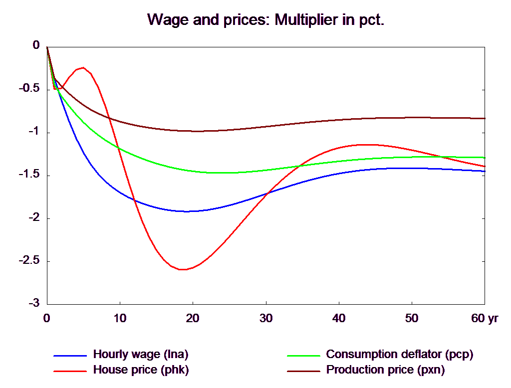
| Wage | lna | -0.36 | -0.63 | -0.86 | -1.06 | -1.23 | -1.70 | -1.87 | -1.91 | -1.84 | -1.71 |
| Consumption price | pcp | -0.44 | -0.58 | -0.69 | -0.79 | -0.88 | -1.19 | -1.36 | -1.45 | -1.47 | -1.43 |
| Terms of trade | bpe | -0.31 | -0.39 | -0.45 | -0.51 | -0.55 | -0.70 | -0.76 | -0.78 | -0.77 | -0.74 |
| Percentage-point | |||||||||||
| Consumption ratio | bcp | -0.06 | -0.10 | -0.01 | 0.03 | 0.06 | 0.00 | -0.13 | -0.20 | -0.21 | -0.20 |
| Wage share | byw | -0.18 | -0.32 | -0.39 | -0.44 | -0.46 | -0.44 | -0.41 | -0.37 | -0.33 | -0.28 |
As the amount of output demanded can be produced by less labor, employment falls already in the first year, and due to lags in the labor demand relation the negative effect on employment peaks in the second year. The lower employment reduces wage growth and the wage-driven crowding out returns employment to its baseline.▼ The wage relation in ADAM is a Phillips curve, which links the changes in wages to unemployment. A fall/rise in unemployment pushes wages and hence prices upward/downward and reduces/improves competitiveness. So exports and production decrease/increase and over time unemployment returns to its baseline. This is the wage-driven crowding out process.
Compared to the previous two experiments - increase in number of workers and working hours, nominal hourly wages fall by a smaller percentage when labor efficiency improves, because production costs fall and make producer prices fall. Therefore, nominal wages do not have to decrease substantially to induce the fall in prices, that is necessary to make net exports increase and offset the initial fall in labor demand. This also explains the quicker response in exports in the present experiment, compared to the previous two experiments. Moreover, in the long run there is only a small negative effect on real hourly wages and there is no effect on private consumption in the long run.
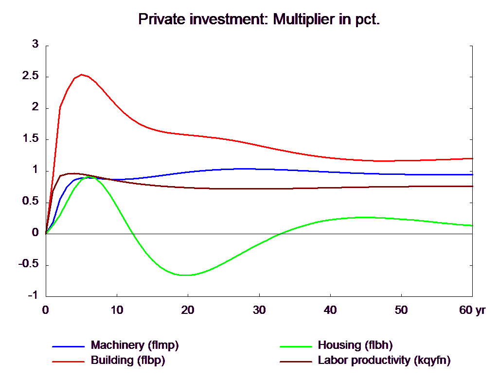
Investments in machinery fall as the improvement in labor efficiency makes labor substitute for machinery. Capital intensity of production falls as production involves less capital and more labor. Due to this fall in capital intensity, output per working hour increases by less than 1 percent despite the 1 percent increase in labor efficiency.
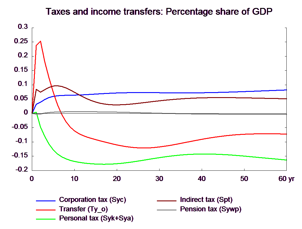
Note that the higher unemployment in the short run raises unemployment benefits and worsens public finance temporarily. Later on the initial worsening in the government budget is reversed and the permanent budget effect is positive as employment rises and tax revenues increase. The improved competitiveness and the additional public savings also enhances the balance of payment.
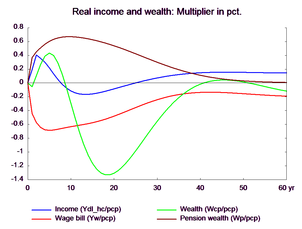
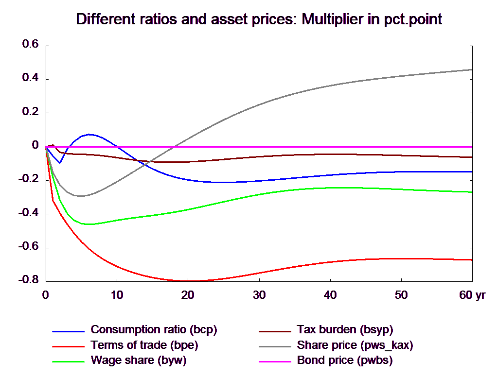
Figure 12. The effect of a permanent 1 percent increase in labor efficiency